What a Simulation Shows About a Decision I Made Without One

In 2022 I exited a data privacy startup I had co-founded. I had a material stake in it after two years. There was friction at the end. I left.

That decision was made on gut, financial pain, and the sense that I was the wrong person in the wrong seat at the wrong time. Not on a model. I didn’t have these tools then.

Four years later, I ran the decision through a structured thinking protocol and a probability model — to find out whether the call was right, and more importantly, what actually drove the outcome. The most useful finding wasn’t in the headline numbers.

---

The finding that surprised me

Not because execution doesn’t matter. Because it’s the last gate in a chain. The regulation must arrive AND the company must still be running AND then execution must be good. Each condition multiplies the others — and the early gates dominate the product.

This is what a probability model surfaces that a narrative argument doesn’t.

---

Before the model: The Blade

Before running any numbers, I ran /critical-thinking — The Blade protocol. Six questions designed to surface what you’re not seeing before you start computing.

The most important output was a framing constraint: this simulation is post-hoc. The decision was made on gut and friction, not analysis. Publishing it as validation of a calculated choice would be dishonest — and that dishonesty would undermine everything the field note claims to show.

The Blade’s cut:

• One thing to do: Frame this explicitly as retrospective. These tools didn’t exist when I decided.
• One thing to stop: No characterization of the people who continued building. The analysis is about the structure of the decision, not the people inside it.

---

The model

Two scenarios. 10,000 runs each. Every input is a probability distribution, not a fixed value.

Scenario A — Exited 2022: Income growth rate, year-over-year growth consistency, capital that stopped burning after exit.

Scenario B — Stayed: Annual cash burn, probability DPDPA enforcement becomes meaningful, probability the company survives long enough to see demand, probability of executing well enough to capture it, size of a blockbuster outcome if all three conditions fire simultaneously.

Measure	Scenario A — Exited	Scenario B — Stayed
Median 4-year net	+12.7× the original stake	−4.7× the original stake
Positive outcome	10,000 of 10,000 runs	160 of 10,000 runs
A dominates B	98.6% of matched runs	—
Model settled	Yes	No — two modes
Median gap	17× the original stake in favour of A	—

Scenario B’s model didn’t settle to a stable mean. That non-convergence is a finding, not a flaw: it is the statistical signature of a two-mode outcome. Almost always bad, rarely transformative, nothing in between. The 1.6% blockbuster tail keeps pulling the average — which is why the median tells you more than the mean here.

---

What drives each outcome

The model can attribute how much of the variance in each scenario is explained by each input. This is where the structure of the bet becomes visible.

In Scenario A, growth trajectory and capital saved together explain nearly all the variance. Starting income explains almost nothing — it gets compounded into irrelevance within two years. The value of exiting depends almost entirely on whether the career compounds, not on what you start earning.

In Scenario B, the three biggest drivers are:

Input	Share of variance
Survival — does the company last long enough to see DPDPA demand?	36%
Blockbuster value — how large is the payoff if everything fires?	29%
Regulatory arrival — does DPDPA enforcement actually materialise?	18%
Burn rate	15%
Execution quality	2%

The people who stayed are not running an execution problem. They are running a timing and survival problem. Improving execution from poor to strong barely moves the distribution — because the other conditions gate it first.

The company’s fate in Scenario B is more clock-dependent than skill-dependent.

---

What this is and isn’t

The model validates the exit with high probability. But that’s not the useful part — the gut had already computed that.

The useful part is structural: the decision wasn’t primarily about whether the team could execute, or whether the regulatory bet would pay off. It was about whether staying in a compounding-loss position while waiting for an external catalyst — one the company doesn’t control — was the right deployment of four years of productive capacity.

The sensitivity breakdown quantifies what the gut was probably computing under pressure: the clock cost dominated, and execution quality barely moved the distribution.

The 1.6% blockbuster scenario is real. Those who stayed are running that bet. The model shows exactly what lever matters most: survival probability, not execution quality.

---

Technical detail — distribution chart

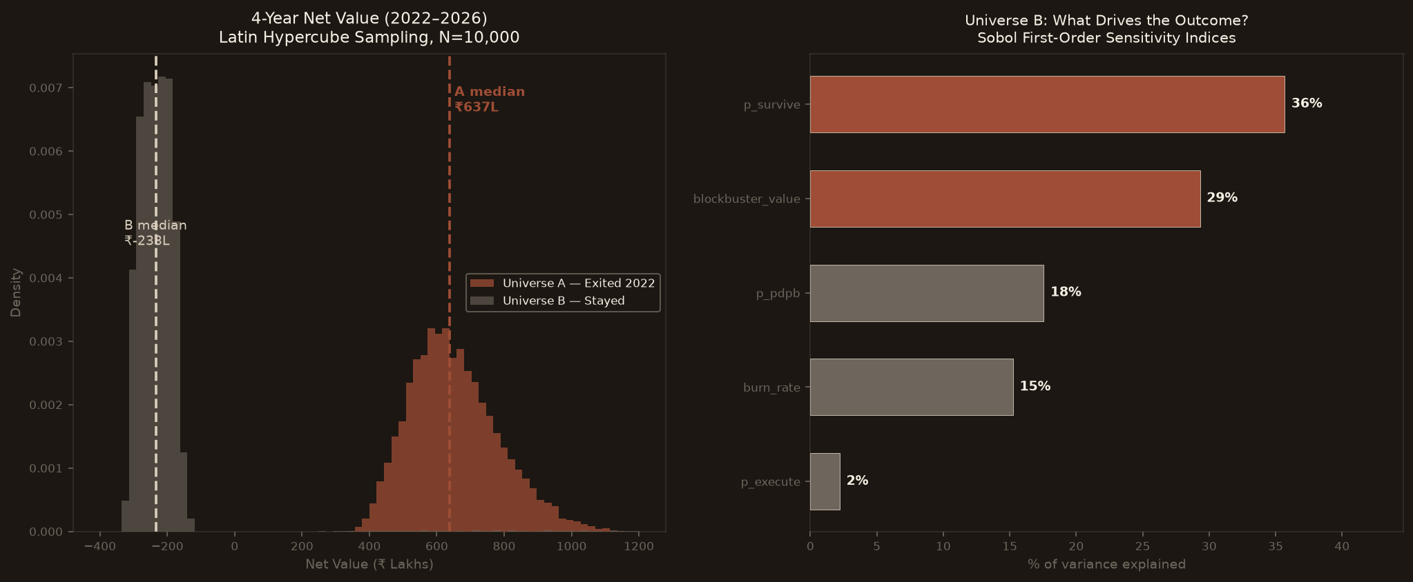
The left panel shows outcome distributions for both scenarios across 10,000 runs using Latin Hypercube Sampling. The right panel shows Sobol first-order sensitivity indices — how much of Scenario B’s variance each input explains independently.

---

Tools: /critical-thinking — The Blade (State / Failure / Unseen / Actors / Constraint / Cut). /monte-carlo — 10,000 runs per scenario, Latin Hypercube Sampling, Sobol first-order sensitivity indices.

All figures are multiples of the original stake. No absolute financial figures.

The Leela.works playbook entry-point analysis — a different decision, same tools — is a separate field note.